|
CA: an application
The well-known Cellular
Automaton (CA) proposed by John von Neumann in the late 1940's can
be regarded as a subclass of Random Boolean Networks. In a CA a
node only receives inputs from nodes in his local neighbourhood
and each node has the same logic transition rule. It is therefore
possible to simulate any CA with the RBN Toolbox just by defining
the network's connections and rules accordingly.
Defining
the Connection-Matrix for a CA
As the future state of a
cell (node) only depends on the actual state of the cell and the
states of its two adjacent cells, the Connection-Matrix is a
band-matrix with exactly three entries per column.
Let's create a Cellular Automaton with 90 cells in a
ring-structure, that is, the first and the last cell of the array
are connected.
>> A = ones(90,90);
>> B = tril(A,-2);
>> C = triu(A, 2);
>> D = B + C;
>> D(1,90) = 0;
>> D(90,1) = 0;
>> D(find(D == 1)) = 2
>> D(find(D == 0)) = 1;
>> D(find(D == 2)) = 0;
>> conn = initConnections(D)
conn now contains the Connection-Matrix for a
90-cells-CA.
Defining the Rules-Matrix for a CA
The Rules-Matrix in our example will be a 2^3 x 90
matrix with identical columns (as each node has the same logic
transition rule). Here the transition rule is defined as follows:
The logic transition
rule for each cell
| State of
neighbouring cell "on the left" |
State of cell
itself |
State of
neighbouring cell "on the right" |
Next State |
| 0 |
0 |
0 |
1 |
| 0 |
0 |
1 |
0 |
| 0 |
1 |
0 |
1 |
| 0 |
1 |
1 |
0 |
| 1 |
0 |
0 |
0 |
| 1 |
0 |
1 |
1 |
| 1 |
1 |
0 |
0 |
| 1 |
1 |
1 |
1 |
The Rules-Matrix is therefore defined as follows:
>> for i=1:90
>> rules(:,i) = [1 0 1 0 0 1 0 1]';
>> end
>> rules = initRules(rules);
Setting the initial states of the
cells
In our example we want all
cells to have their initial state set to 1, except for cell number
46, which is set to 0.
>> initialStates = ones(90,1);
>> initialStates(46) = 0;
Creating the Node-Structure-Array
and visualizing the topology
Before running the evolution, we
have to create
the Node-Structure-Array by calling some initialising functions
with the previously prepared matrices as parameters.
>> node = initNodes(90,initialStates,zeros(90,1),zeros(90,1));
>> node = assocRules(node, rules)
>> node = assocNeighbours(node,conn);
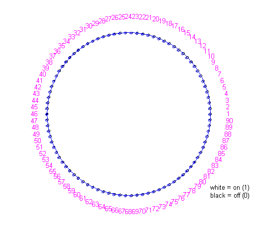
>> node = displayTopology(node, conn, 'line');
As a result we get the
visualization of the topology of our Cellular Automaton.

Displaying the evolution
Classically, in a CA all
cells are updated at each time step, so the appropriate RBN update
mode is cleary the CRBN
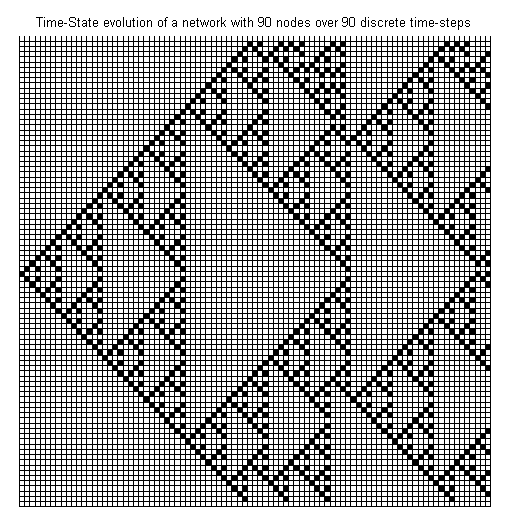
update mode. The evolution of our CA over 90 discrete
time-steps is launched with:
>> [node, tsm] = displayEvolution(node, 90, 'CRBN');
The visualization of the
evolution yields a intricate nested pattern, which is typical for
Cellular Automata ([B3]).

|